What Drives Equity Returns?
Total equity returns can be approximated as the sum of earnings growth, changes in valuation (P/E), and dividends:
A) Earnings Growth (Structural Driver)
-
-
-
- Definition: Growth in earnings per share (EPS)
- Source: Revenue growth, margins, productivity
-
-
Over long horizons, EPS growth tends to track nominal economic growth (real growth + inflation). This is the only truly durable driver of long-term returns.
B) Multiple Expansion / Contraction (Valuation)
-
-
-
- Definition: Change in the price investors are willing to pay per dollar of earnings (P/E)
- Driver(s): Interest rates, inflation, and risk appetite
- Falling rates / low inflation → higher multiples
- Rising rates / uncertainty → lower multiples
-
-
Over short horizons, valuation changes can dominate returns. Over longer periods, they tend to mean revert, leaving earnings as the primary driver.
C) Dividends (Cash Return)
-
-
-
- Definition: Cash returned to shareholders
- Role: Stable contributor to total return
-
-
Dividends have historically contributed a meaningful portion of total returns, though their role has declined with the rise of share buybacks, which now serve as a primary mechanism of capital return.
- Short Term vs. Long Term: In any single year, multiple expansions can easily be the biggest driver of returns (it outpaced earnings in 18 of the last 35 years). However, over the decades, those sentiments often cancel each other out, leaving earnings and dividends as the only permanent gains.
- Risk of “Multiple Contraction”: If a stock’s price rose mainly because of a high P/E ratio (multiple expansion) rather than profit growth, it is fragile. If sentiment cools or interest rates rise, that multiple can “compress,” causing the stock price to crash even if the company’s earnings remain stable
The Anchor: Equity Risk Premium (ERP)
Definition
ERP = Expected Equity Return − Risk-Free Rate
In practice, we approximate ERP using earnings yield as a valuation proxy, recognizing that true expected returns also depend on future growth. This metric represents the extra return investors expect to earn from the expected stock market (S&P500) return over a “risk-free” asset like a 10-year Treasury note. Think of it as an insurance gauge. The higher the perceived risk in stock returns, the higher the ERP.
Two Ways to Think About ERP
1) Implied ERP (Valuation Spread)
ERP_proxy = Earnings Yield – Risk-free rate
-
-
- Uses forward (NTM) earnings
- Captures a snapshot valuation spread vs bonds
-
Interpretation:
-
-
- Low ERP → equities expensive relative to bonds
- High ERP → equities cheap relative to bonds
-
This is a short-term valuation metric, not a full return estimate.
2) Expected ERP (Total Return Framework)
ERP_expected = (Earnings Yield + g) – Risk-free rate
Where:
-
-
- g = long-term earnings growth (proxied by Nominal GDP (nGDP))
-
Interpretation:
-
-
- Captures expected long-term return compensation
- Aligns with how equities compound over time
-
Key Distinction:
| Metric | What it Measures | Time Horizon |
| Implied ERP | Valuation spread | Short-term |
| Expected ERP | Expected return | Long-term |
Growth: The Second Pillar
Expected equity returns are not just about valuation—they depend on growth.
Expected Return ≈ Earnings Yield + Earnings Growth
Over long horizons:
Earnings Growth ~ Nominal GDP (nGDP)
But the composition matters critically:
| Component | Mechanism | Market Impact |
| Real Growth | Higher real cash flows | Supports multiples |
| Inflation | Higher discount ratesThe interest rate used to determine what a future sum of money is worth today. It accounts for the "time value of money"—the principle that a dollar today is worth more than a dollar tomorrow—and the risk that a future payment might not actually be received. More | Compresses multiples |
-
-
- Real growth-driven expansion → supports higher multiples
- Inflation-driven growth → compresses multiples
-
Critical Insight:
Not all growth is equal. Markets reward real growth, but penalize inflation-driven growth.
Valuation Framework
At its core, equity valuation follows a Gordon Growth Model (DCF) -type relationship:
Where:
-
-
-
- r = Required return = Risk-Free Rate + ERP
- g = Long-term earnings growth
-
-
This relationship assumes a steady-state environment where growth is stable and below the required return.
Implications
-
-
-
- ↑ Interest Rates → ↑ r → ↓ P/E
- ↑ ERP (risk aversion) → ↓ P/E
- ↑ Growth (real, not inflation) → ↑ P/E
-
-
How Rates Drive the Market
The 10-year Treasury yield is the critical transmission mechanism.
-
- When Rates Rise
-
- Discount rateThe interest rate used to determine what a future sum of money is worth today. It accounts for the "time value of money"—the principle that a dollar today is worth more than a dollar tomorrow—and the risk that a future payment might not actually be received. More increases
- ERP may rise (if risk increases)
- Multiples compress → equities fall
-
- When Rates Fall
-
- Discount rateThe interest rate used to determine what a future sum of money is worth today. It accounts for the "time value of money"—the principle that a dollar today is worth more than a dollar tomorrow—and the risk that a future payment might not actually be received. More declines
- ERP may compress (confidence improves)
- Multiples expand → equities rise
-
- When Rates Rise
Important Nuance
The impact of rising rates depends on why they are rising:
-
-
- Growth-driven increases → ERP may fall (bullish offset)
- Inflation or risk-driven increases → ERP may rise (bearish reinforcement)
-
Why “Bad News Can Be Good News”
Weak economic data can lead to:
-
-
- Lower expected policy rates
- Falling bond yields
- Lower discount ratesThe interest rate used to determine what a future sum of money is worth today. It accounts for the "time value of money"—the principle that a dollar today is worth more than a dollar tomorrow—and the risk that a future payment might not actually be received. More
-
→ Supporting equity valuations even as fundamentals weaken
The Role of ERP in Market Regimes
ERP is best understood as a regime indicator:
-
- Low ERP Environment
-
- Strong confidence
- Stable macro backdrop
- High valuations
- Vulnerable to shocks
-
- High ERP Environment
-
- Fear / uncertainty
- Tight financial conditions
- Lower valuations
- Higher forward return potential
-
- Low ERP Environment
Why Would Investors Accept a Lower ERP?
Investors accept a lower ERP when they are optimistic, certain (complacent), have no better options, or are considering share buybacks.
-
- High Growth Confidence (The “Earnings Engine”)
- If investors believe earnings will grow at a high rate (the current analyst forecast is at 14%), they will accept a thin margin of safety now for massive growth in the future.
- Logic: They’ll take a small ERP (say 4%) over the 10yr today because they’re certain the S&P500 will be far more profitable a year from now.
- “TINA” (There Is No Alternative)
- Investors look at alternatives. Even if they feel the current ERP is low, if they believe inflation will stay sticky at 3-4%, sitting in cash or 10yr (yielding 4.44%) feels like losing money in “real” terms.
- Logic: Risk-Free rate is 4.44%, and inflation is running 3%, but may go higher. Stocks may be the only asset class that can actually outrun inflation through pricing power.
- Low Perceived Macro Risk (Complacency)
- When the economy feels stable (a “Soft Landing”), the perceived risk of a 2008-style crash feels improbable. When fear is low, the price of “insurance” (ERP) drops.
- The indicator: Look at the VIX. When the VIX is low (12–15), investors are comfortable accepting a lower ERP. When the VIX spikes, they suddenly demand a 6% or 7% ERP to stay in the game. As of April 23, 2026, the VIX is at 19.31 after having spiked up in recent weeks due to the Israel/US – Iran conflict.
- Massive Share Buybacks
- In the modern S&P 500, companies are returning record amounts of cash via buybacks. This acts as a “stealth” return.
- Logic: If a company grows at 5% but buys back 3% of its shares, the EPS grows at 8%. Investors accept a lower “base” ERP because they know the buybacks are artificially boosting their per-share value.
- High Growth Confidence (The “Earnings Engine”)
Nominal GDP
Nominal GDP is the market value of all finished goods and services produced and is the sum of Real GDP and Inflation. It can also be a bit misleading, as it can be positive purely due to rising prices (inflation) even if the actual volume of production (Real GDP) remains flat.
As an example, if Nominal GDP is 5% but Real GDP is 0.0%, that means that Inflation is +5%. This is a stagflation-like configuration, and it was what the US experienced in the 1970’s. Even if earnings match inflation, P/E multiples will contract severely as investors will not value “inflation-driven” earnings as highly as “real growth-driven” earnings. Consequently, markets price in a higher implied ERP that entices investors to keep their money in stocks.
- This brings 2025 Nominal GDP (in dollar terms) to $30.762 Trillion
Growth rate (Nominal GDP) – The estimation of Nominal GDP (nGDP) for 2026 is just that, an estimation. (It is cyclical and not a stable long-term equilibrium growth rate.)
Here is my calculation:
-
-
- 2025 nGDP (U.S. BEA) = $ 30.762 Trillion
- 2026 nGDP Estimates (Philadelphia Fed Survey) = $ 32.441 Trillion
- Δ nGDP estimate = 5.46%
-
Earnings Yield, & ERP
- Earnings Yield = 1 ÷ 20.9* {FactSet Earnings Insight || April 17, 2026} = 4.78%
- EPS Estimates marked higher to $336.02. {FactSet S&P500 rate = 7022.95 || April 17, 2026}
- Risk-Free Rate = 4.32%
Implied ERP = 4.78% – 4.32% = 0.46%
*Expected ERP = 4.78% + 5.46% – 4.32% = 5.92%
Using short-term growth expectations (cyclical) in a long-duration valuation model can overstate fair value. The reason is that it is discounting growth twice in the first year. Forward (ntm) estimates already incorporate economic growth and adding nominal GDP estimate to this is a partial overlap between near-term earnings expectations and macro growth assumptions. This post uses this to illustrate the conceptual difference between Implied ERP and Expected ERP. For greater accuracy, analysts use historical long-term equilibrium growth rate averages. The nominal GDP average for the past ~50yrs is between 6% – 6.5%.
Why this Matters
-
-
- Valuation: Current readings place it in the “Extreme Compression” range, indicating that markets are pricing near-perfect conditions, which often coincides with higher P/E ratios (currently around 20.9x forward earnings).
- Asset Allocation: In theory, the higher the ERP, the stronger the “case for stocks”. However, in reality, extremely ERP levels weaken the “case for stocks” relative to bonds. This has to do with investor psychology as much as anything. The returns from “safe” Treasuries become more appealing to investors than the rising ‘insurance’ they would require to stay in stocks. This is not set in stone; just that the ‘Risk Premium’ part of ERP rising suggests investors’ requirements for staying in stocks have risen.
-
-
- The correlation between ERP and Earnings Yield is fairly linear:
-
-
- If investors demand a higher ERP (insurance) to own stocks and (holding Rf Rate constant):
- Earnings Yield is higher ⇒ P/E(nTm) is lower: If Earnings estimates stay constant, then the S&P500 price has to be lower.
- If investors are willing to accept a lower ERP to own stocks (holding Rf Rate constant):
- Earnings Yield is lower ⇒ P/E(nTm) is higher: If Earnings estimates stay constant, then the S&P500 price has to be higher.
- If investors demand a higher ERP (insurance) to own stocks and (holding Rf Rate constant):
-
Economic Scenario ERP Target (%) Earnings Yield (%) Risk-Free Rate(%) P/E (nTm) EPS Est. (nTm) S&P value Return (%)
4/15/2026 0.50 4.78 4.28 20.9 $336 7022 0
Higher ERP 0.75 5.03 4.28 19.9 $336 6686 -4.78
Lower ERP 0.25 4.53 4.28 22.08 $336 7419 5.65
How Interest Rate Changes Affect the S&P 500
Changing interest rates directly alters the required return (discount rateThe interest rate used to determine what a future sum of money is worth today. It accounts for the "time value of money"—the principle that a dollar today is worth more than a dollar tomorrow—and the risk that a future payment might not actually be received. More) for equities.
-
-
- Higher rates → higher required return → lower P/E → lower index level
- Lower rates → lower required return → higher P/E → higher index level
-
Crucially, equity markets adjust prices to maintain a risk premium (ERP) over risk-free assets.
If Treasury yields rise and ERP is unchanged, equity prices must fall to restore that spread.
If yields fall, equities can re-rate higher even without changes in earnings.
S&P 500 Sensitivity Analysis
Baseline Assumptions:
-
-
- EPS (NTM): $336
- Long-term growth (g): ~5.46% (nominal GDP proxy)
- Framework: Gordon Growth approximation
-
P/E = 1 ÷ ((Risk-free rate + ERP) – g)
-
-
- Index Level = EPS × P/E
-
⚠️ Important Clarification
The ERP used below reflects a full expected return framework (including growth) and is therefore higher than the simplified earnings-yield-based ERP proxy shown earlier.
| 10-yr Yield | 4.5% ERP | 5.0% ERP | 5.5% ERP | 5.92% ERP (4/23/2026) | 6.0% ERP | 6.5% ERP |
|---|---|---|---|---|---|---|
| 3.50% | 13228 Goldilocks | 12,500 | 10,458 | 8485 | 7,824 | 7,018 |
| 3.75% | 12043 | 10213 | 8865 | 7981 | 7832 | 7015 |
| 4.0% | 11053 | 9292 | 8317 | 7534 | 7401 | 6667 |
| 4.25% | 10213 | 8865 | 7832 | 7134 | 7015 | 6352 |
| 4.32% (4/23/2026) | 10000 | 8705 | 7706 | 7029 | 6914 | 6269 |
| 4.50% | 9492 | 8317 | 7401 | 6774 | 6667 | 6065 |
| 4.75% | 8865 | 7832 | 7015 | 6449 | 6352 | 5803 |
| 5.0% | 8317 | 7401 | 6667 | 6154 | 6065 | 5563 |
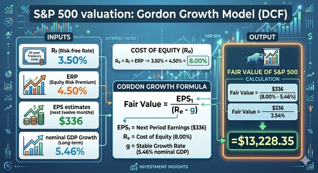
Gordon Growth Model (DCF)
“Goldilocks” Calculation
When (Risk-free rate +ERP) approaches g, valuations expand nonlinearly. This is the “Goldilocks zone.”
If 10-Year Yield drops to 3.5% and the ERP falls to 4.5% while long-term equilibrium growth stays constant, the market enters a high-valuation “Goldilocks” zone. Here is the “Fair Value (FV)” math:
-
-
- The “Spread” is key: The denominator in this formula isn’t just the interest rate; it’s the gap between the total required return (8.0%) and the long-term equilibrium growth rate estimate (5.46%).
- Huge FV swings: Because that gap is so small (only 2.54%), even a tiny 0.25% change in interest rates or growth expectations causes the “Fair Value” to swing by thousands of points.
- The Bull Case: This calculation shows why markets rally so hard when rates fall. By dropping the 10-year yield from its current ~4.32% to 3.5% and gaining confidence (lowering ERP), the “justifiable” price for the S&P 500 almost doubles.
-
Putting It All Together
Expected Equity Return
Valuation Constraint
Key Macro Takeaways
- Rates set the valuation ceiling
-
- Higher yields increase the required return → compress multiples
-
- ERP reflects fear, not opportunity (directly)
-
- High ERP = risk is elevated
- Low ERP = risk is underpriced
-
- Growth quality matters more than growth level
-
- Real growth → bullish
- Inflation → bearish for multiples
-
- Short-term vs long-term drivers
-
- Short-term: rates + ERP (multiples)
- Long-term: earnings growth
-
Bottom Line
Equity markets are governed by a simple but powerful interaction:
Valuation (rates + ERP) × Growth (quality matters)
- Rates and risk determine what investors are willing to pay
- Growth determines what they are paying for
When these diverge—that’s where opportunity and risk emerge.